Numerical Dynamics in Practice: Euler to RK4, Van der Pol, and N-Body Orbits

Numerical methods for ODEs are one of those subjects where the theory reads cleanly on the page and then punishes you the moment you try it on anything non-trivial. This post walks through three problems I worked on for a numerical analysis course, each less forgiving than the last, and what the numerics actually do once you turn the crank.

The methods

All three problems use the same three integrators. Given a state $x$ , a vector field $f$ , and step size $h$ , each one advances a step as follows.

Forward Euler, one slope and one step:

x_{n+1} = x_n + h\, f(x_n)

Modified Euler (Heun's method), the average of two slopes:

x_{n+1} = x_n + \tfrac{1}{2}(k_1 + k_2), \quad k_1 = h f(x_n),\ k_2 = h f(x_n + k_1)

Classical fourth-order Runge–Kutta (RK4), four weighted slopes:

x_{n+1} = x_n + \tfrac{1}{6}(k_1 + 2k_2 + 2k_3 + k_4)

where $k_1, k_2, k_3, k_4$ are successive slope estimates along the step. The global error scales as $O(h)$ , $O(h^2)$ , and $O(h^4)$ respectively, a gap that looks innocuous on paper and enormous in practice.

Problem 1: exponential growth

Start with the simplest possible test case:

x' = x, \quad x(0) = 1

The exact solution is $x(t) = e^t$ , so $x(1) = e \approx 2.7183$ . Running each method with $h = 0.1$ (ten steps) to $t = 1$ :

| Method | Approx | Error | |---|---|---| | Euler | 2.593742 | $1.25 \times 10^{-1}$ | | Modified Euler | 2.714081 | $4.20 \times 10^{-3}$ | | RK4 | 2.718280 | $2.08 \times 10^{-6}$ |

Euler is off by about $0.125$ , which is typical first-order behaviour. Modified Euler drops the error by roughly two orders of magnitude. RK4 hits six-digit accuracy in ten steps. On a smooth exponential, the order of the method is the whole story.

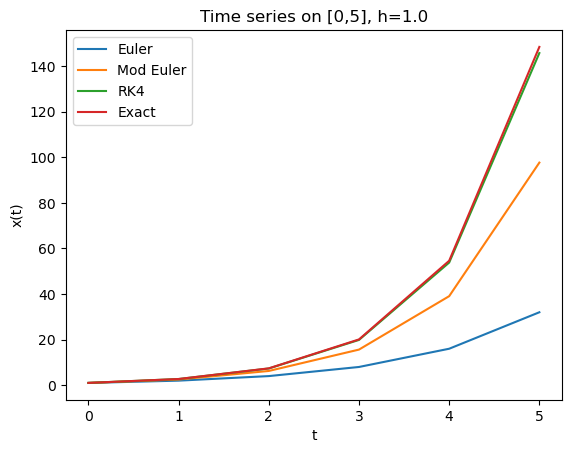
Extending to $t = 5$ with different step sizes makes the gap between methods visible. At $h = 1.0$ , Euler lags far below the exact curve while RK4 overlaps it almost exactly:

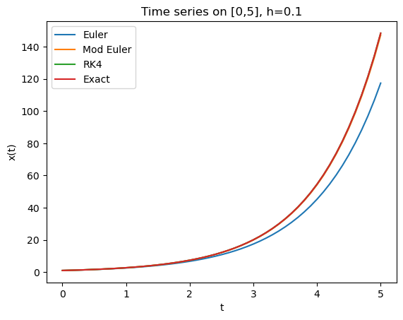
Time series comparison at h=1.0 — Euler badly undershoots the exponential, while RK4 tracks it exactly.

At $h = 0.1$ , modified Euler and RK4 both overlap the exact solution and only Euler shows visible error:

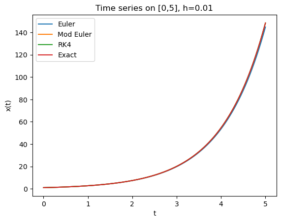
Time series at h=0.1 — only Euler deviates from the exact solution.

By $h = 0.01$ , all four curves are indistinguishable:

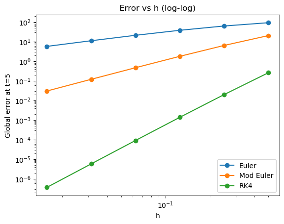
Time series at h=0.01 — all methods converge to the exact solution.

The log–log error plot confirms the convergence rates quantitatively. The slopes are $1$ , $2$ , and $4$ . Halving $h$ halves Euler's error, quarters modified Euler's, and cuts RK4's by a factor of sixteen:

Log-log plot of global error vs step size h, showing slopes 1, 2, and 4 for the three methods.

Problem 2: the Van der Pol oscillator

The Van der Pol equation is a non-conservative oscillator with nonlinear damping:

x'' - \mu(1 - x^2)x' + x = 0

Introducing $y = x'$ turns it into a first-order system:

x' = y, \qquad y' = \mu(1 - x^2)y - x

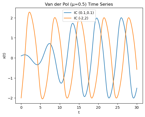
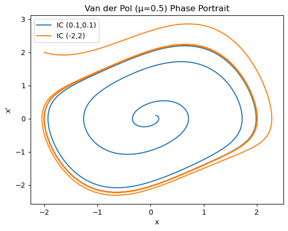
For $\mu = 0.5$ , the system has a stable limit cycle. I integrated it with RK4 from two very different initial conditions, $(0.1, 0.1)$ and $(-2, 2)$ . The time series shows both trajectories settling into the same regular oscillation after about ten time units:

Van der Pol time series at mu=0.5, showing two different initial conditions converging to the same oscillation.

The phase portrait makes the point more cleanly. Both trajectories spiral onto the same closed loop. That is what a limit cycle means: the system forgets where it started.

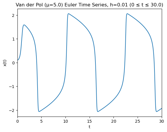
Van der Pol phase portrait at mu=0.5, showing the stable limit cycle with both ICs converging to a single closed orbit.

Things get more interesting at $\mu = 5$ , where the oscillator becomes stiff. It spends most of its time drifting slowly and then executes a sharp jump. With explicit Euler at $h = 0.01$ the relaxation oscillation is clearly visible: slow decay through zero, rapid jump to $x \approx 2$ , repeat:

Van der Pol stiff time series at mu=5, h=0.01, showing sharp relaxation oscillations.

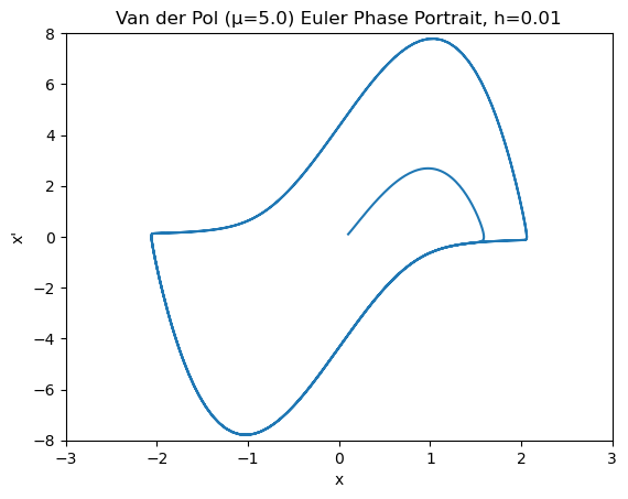
The phase portrait at this step size traces the egg-shaped limit cycle with its characteristic sharp corners at the fast jumps:

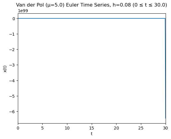
Van der Pol stiff phase portrait at mu=5, h=0.01, showing the egg-shaped limit cycle.

Push the step size to $h = 0.08$ and the solution blows up to order $10^{99}$ in a handful of steps. The limit cycle is gone:

Van der Pol blowup at mu=5, h=0.08 — the solution shoots to 1e99 and the time series flatlines.

The phase portrait never closes. The trajectory spirals out wildly before escaping to infinity:

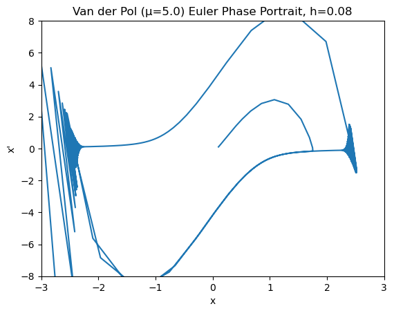
Van der Pol phase portrait at mu=5, h=0.08 — chaotic divergence, no closed orbit.

That is the practical meaning of stiffness. A method that works fine on smooth problems can fail catastrophically when the system has sharp transitions, and the cure is not always a higher-order method. Often it is just a smaller step, or an implicit scheme.

Problem 3: gravitational N-body orbits

For $n$ planets interacting gravitationally, Newton's laws give $6n$ first-order ODEs:

r_i' = v_i, \qquad v_i' = \sum_{j \neq i} G m_j \frac{r_j - r_i}{\|r_j - r_i\|^3}

Packing the state into a NumPy array of shape (n, 2, 3), with one slot per body for position and one for velocity, each a 3-vector, lets the same rk4 routine handle the two-body and three-body cases without modification.

Two bodies

With $m_0 = 1$ , $m_1 = 2$ , RK4 produces clean closed ellipses. The lighter body traces the larger ellipse, the heavier body the smaller one, and the centre of mass stays pinned at the origin:

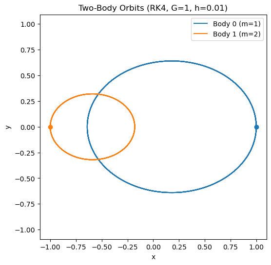
Two-body orbits computed with RK4 — the lighter body (m=1) traces the larger ellipse.

Conservation laws the integrator was never told about fall out for free, because RK4 is accurate enough over twenty time units that the drift is invisible to the eye.

Three bodies: the figure-eight

The three-body problem has no closed-form solution in general, but it does admit remarkable periodic orbits where three equal masses chase each other along a shared curve. The most famous is the figure-eight, discovered by Moore (1993) and Chenciner–Montgomery (2000). With parameters

a = 0.347111, \quad b = 0.532728, \quad T \approx 6.324449

the three trajectories trace out a single figure-eight curve:

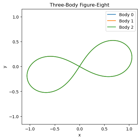
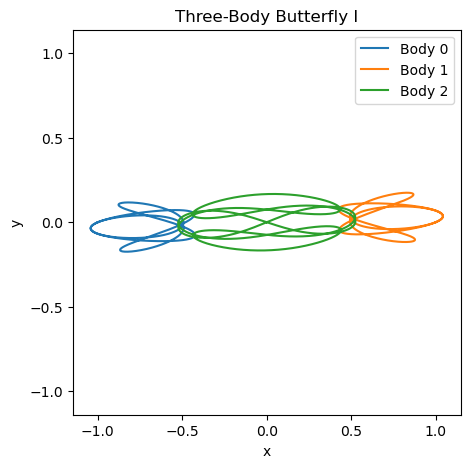
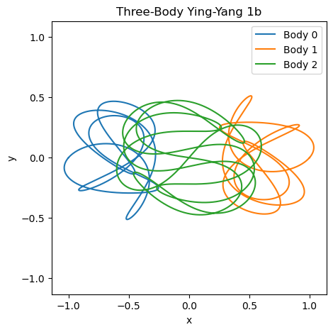
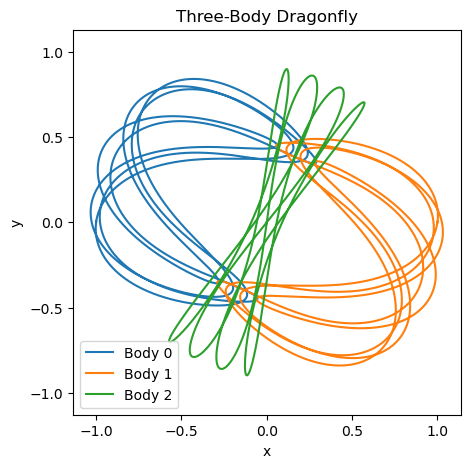
Three-body figure-eight orbit — three equal masses chasing each other along a single closed curve.

Other known three-body orbits work the same way. Pick the right $(a, b, T)$ and the integrator draws the pattern. These runs need a much smaller step (I used $h = 5 \times 10^{-5}$ ) because small integration errors accumulate over the long period.

Three-body Butterfly I orbit.

Three-body Ying-Yang 1b orbit.

Three-body Dragonfly orbit.

What I took away

The tidy version of the story is that higher-order methods beat lower-order methods. That is true on smooth problems and visible within ten steps of an exponential. The less tidy version is that order of accuracy is only part of what determines whether a method is useful. Stiffness kills explicit methods regardless of order. Long-horizon problems, orbits especially, punish any method that fails to preserve the right geometric structure, which is why symplectic integrators exist and why even RK4 eventually drifts.

The full code lives in the course assignment. The point of writing it up here was less about the Python and more about what the plots taught me. Every method has a regime where it is the right tool. The skill worth developing is recognising which regime you are in.