The Curse of Dimensionality

"In high dimensions, your intuition is not just wrong. It is confidently, systematically, and entertainingly wrong."

I spent most of last term staring at a 216-dimensional dataset for my dissertation. Every day of Great Britain's electricity grid, compressed into a single row: demand, prices, wind, solar, temperature. Every time I reached for something from a second-year statistics module, the result came back wrong in a way that was hard to argue with. Distances collapsed. Covariance matrices refused to invert. The nearest neighbour of a point was no longer meaningfully nearer than the furthest.

People call this the curse of dimensionality, which makes it sound like a single phenomenon. It is not. It is a loose family of related failures, each one a place where geometry you trusted in three dimensions stops applying in fifty. What follows are the ones I found hardest to accept, written down in roughly the order I had to confront them.

1. What people mean when they say "high-dimensional"

Fix notation first. We have $n$ observations and $d$ features, giving a data matrix $X$ of size $n \times d$. The classical statistics I grew up on assumed $d$ was small and $n$ was large. 200 patients, 4 measurements. In that regime the sample mean is close to the true mean, the sample covariance is close to the true covariance, and intuition does most of the work for you.

"High-dimensional" just means we have left that regime. It does not require $d$ to be enormous in absolute terms; it requires $d$ to be large relative to $n$. Genomics often has $n = 100$ patients and $d = 20{,}000$ genes. My dissertation had $n = 1{,}819$ days and $d = 216$ hourly features. That is not extreme, but it is already well past the point where the familiar machinery quietly gives up. Here is why.

2. The sample covariance matrix has a rank ceiling

Almost every classical multivariate method, from Mahalanobis distance to linear discriminant analysis to the multivariate Gaussian log-likelihood, requires you to invert the sample covariance matrix $S$. There is a clean lemma that tells you when this is even possible.

Lemma. Let $X$ be an $n \times d$ data matrix and $S = X'HX / (n-1)$ the usual sample covariance, where $H = I - (1/n)\mathbf{1}\mathbf{1}'$ is the centering matrix. Then $\text{rank}(S) \leq \min\{d, n-1\}$. In particular, $S$ is singular whenever $d \geq n$.

The proof is almost a one-liner once you see it. The centering matrix $H$ is an orthogonal projector onto the mean-zero subspace, so it has rank $n - 1$. Writing $Z = HX$, we get $(n-1)S = Z'Z$, and $\text{rank}(Z'Z) = \text{rank}(Z) \leq n - 1$. If $d$ exceeds $n - 1$, the column space simply cannot fit that many directions, and at least $d - (n - 1)$ eigenvalues of $S$ are forced to be exactly zero.

Zero eigenvalues mean $S$ is not invertible. No inverse means no Mahalanobis distance and no Gaussian log-likelihood. An entire tradition of likelihood-based multivariate inference quietly rests on an assumption that fails the moment your data is wider than it is tall.

3. Watching the spectrum collapse

This is the part of my dissertation I had to see to believe. Fix $n = 100$ observations. Draw them from a $d$-dimensional standard normal, so the true covariance is the identity and every eigenvalue should be exactly 1. Now vary $d$ and look at the eigenvalues of the sample covariance.

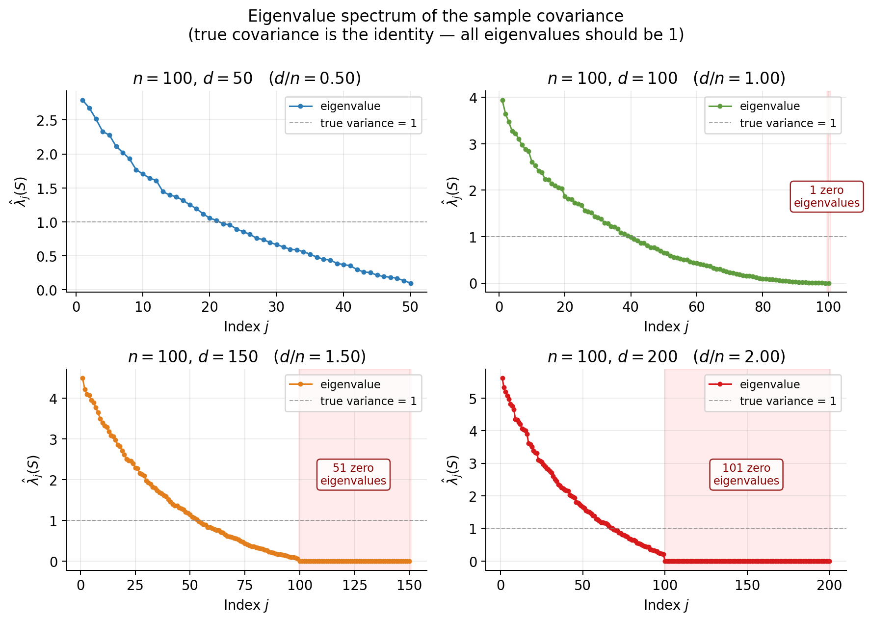
Figure 1. Sample covariance eigenvalues with n = 100 fixed. The true eigenvalues are all 1 (dashed line). As d grows past n−1 = 99, the tail of the spectrum collapses to exact zero, in quantities predicted by the rank lemma.

At $d = 50$ (top-left), every eigenvalue is positive, but instead of clustering around 1 the largest sits near 3 and the smallest near 0. That is finite-sample noise inflating the spread. No singularity yet, but the condition number is already poor.

At $d = n = 100$ (top-right), the rank bound forces exactly one zero eigenvalue. Push further to $d = 150$ and $d = 200$ and the shaded red tail contains 51 and 101 zero eigenvalues respectively, matching $d - (n-1)$ to the exact count.

Here is the R code that produced those panels, lightly edited from what ended up in my dissertation:

set.seed(3772)
n <- 100
d_grid <- c(50, 100, 150, 200)

for (d in d_grid) {
  X <- matrix(rnorm(n * d), nrow = n, ncol = d)
  Xc <- scale(X, center = TRUE, scale = FALSE)
  S <- crossprod(Xc) / (n - 1)
  eigs <- eigen(S, symmetric = TRUE, only.values = TRUE)$values
  n_zero <- sum(eigs < 1e-10)
  cat(sprintf("d = %3d : %d zero eigenvalues\n", d, n_zero))
}

Run it. You get 0, 1, 51, 101. The algebra is not abstract. It shows up in numpy and R as reliably as a compiler error.

The damage starts well before d = n

The subtlety I was slow to appreciate is that the lemma only tells you when $S$ is singular, not when $S$ is useful. A matrix can be technically invertible while being numerically worthless, in the sense that tiny perturbations of the input produce enormous changes in the inverse. The standard measure for this is the condition number: the ratio of the largest eigenvalue to the smallest.

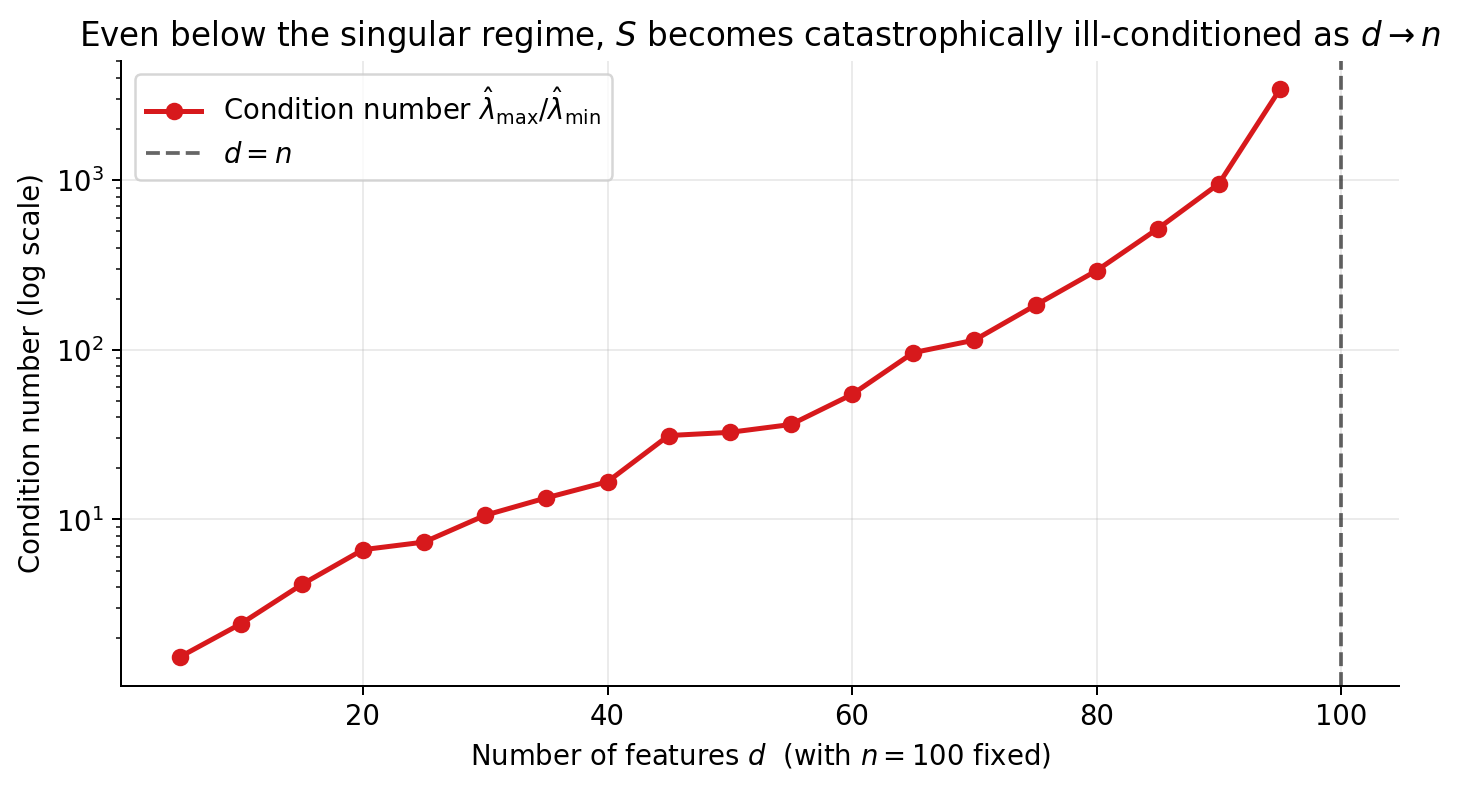
Figure 2. Condition number of the sample covariance with n = 100 fixed, as d increases. Note the log scale. By d = 95 --- still below the singular threshold --- the condition number has exploded by nearly four orders of magnitude.

At $d = 10$ the condition number is a sensible 3 or 4. By $d = 95$ it has already crossed 1,000. Anything you invert in that regime is, for practical purposes, a random matrix with a handful of well-estimated directions and a long tail of numerical noise. The cliff at $d = n$ is dramatic, but it is where the problem ends, not where it begins.

4. Geometry betrays you too

The covariance story is the cleanest mathematical statement of the curse. The stranger parts are about shapes. I want to show two that my second-year self would have refused to believe.

Volume hides near the surface

Take a solid ball of radius 1 in $d$ dimensions. What fraction of its volume sits in the outer shell between radius $0.99$ and $1$? In 3D, almost nothing, about 3%. In 100D, more than 63%. In 500D, essentially all of it.

The calculation is embarrassingly short. The inner ball of radius $1 - \varepsilon$ has volume proportional to $(1 - \varepsilon)^d$ relative to the full ball, so the fraction sitting in the outer shell is $1 - (1 - \varepsilon)^d$. For any fixed $\varepsilon > 0$ that races to 1 as $d$ grows.

Everything is equidistant

Scatter points uniformly in a $d$-dimensional cube. In low dimensions some pairs are close and some are far, and the ratio of the largest pairwise distance to the smallest is large. As $d$ grows, that ratio collapses toward 1. Every pair of points ends up roughly the same distance apart.

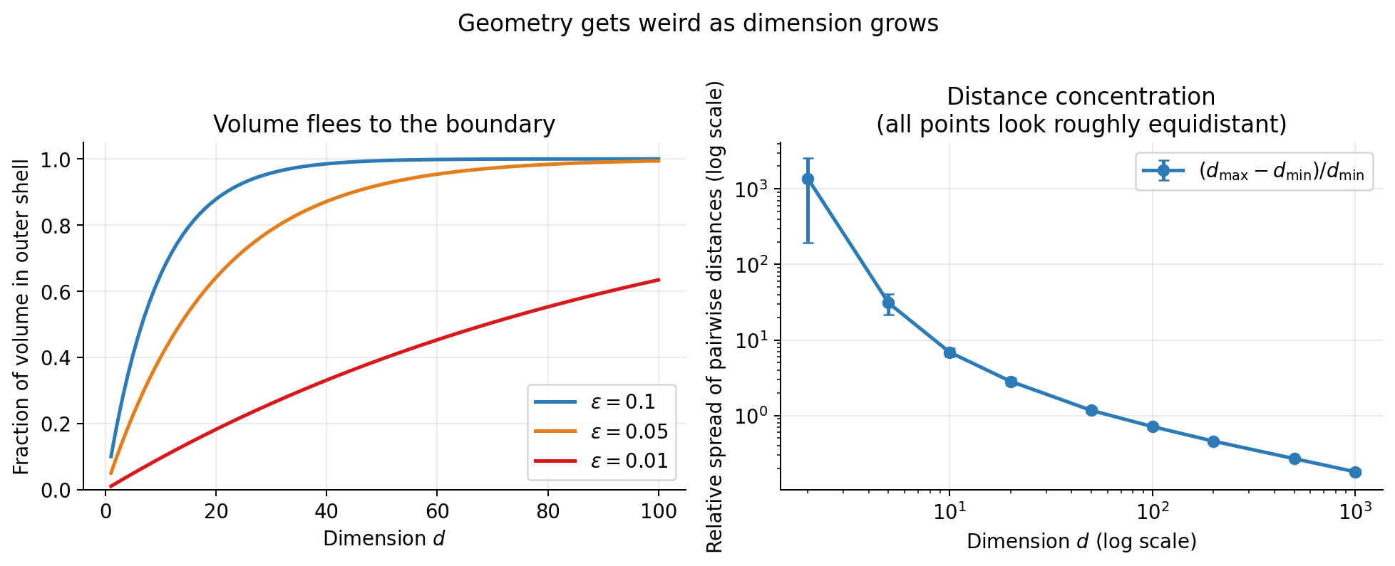
Figure 3. Left: fraction of the unit ball's volume inside the outer shell of thickness $\varepsilon$. Right: the relative spread of pairwise distances between uniformly scattered points. As d grows, points cluster near the boundary, and pairwise distances become nearly identical.

At $d = 2$, the maximum pairwise distance is about 1,000 times the minimum. By $d = 1{,}000$, it is less than 1.2 times the minimum. "Nearest" neighbour has quietly become an almost meaningless concept. Any two points are about as close as any other two.

The consequence is sobering. Similarity is the foundation of k-nearest-neighbour classification, of most clustering, and of most retrieval algorithms. In high-dimensional ambient space it stops meaning what you think it means, and throwing more features at the problem does not rescue the tool.

5. So what do we actually do?

The honest answer is that we either regularise or we reduce dimension. Usually both.

Regularise

If we refuse to give up on the full $d$-dimensional covariance, we can replace $S$ with a shrinkage estimator, a weighted blend of $S$ and some well-conditioned target $T$:

$$\tilde{S} = (1 - \alpha) S + \alpha T$$

Ledoit and Wolf (2004) showed how to pick $\alpha$ optimally in a mean-squared-error sense. The resulting estimator is always invertible, always better-conditioned, and often has lower risk than $S$ itself even at moderate $d$. It is the single most useful technical fix I know of for the covariance problem.

Reduce dimension

The alternative, which is what I spent my dissertation on, is to stop working in $d$ dimensions at all. The observation behind dimension reduction is that real-world high-dimensional data is rarely truly high-dimensional. My 216 hourly features were heavily redundant. Temperature at noon is highly correlated with temperature at 2pm. Solar generation tracks radiation. Wind at different hours moves together. The effective dimensionality was much lower than 216.

Principal Component Analysis is the classical answer. It finds an orthogonal transformation into axes ordered by how much variance they capture. For the energy data, two components captured 55% of the variance and seventeen captured 90%. I went from 216 dimensions to 17 without losing much of the signal.

PCA has a beautiful structure: the principal components are eigenvectors of the sample covariance, and the variance they explain is the corresponding eigenvalue. It also inherits every limitation of $S$. It is a linear method, and if the true structure of your data lies on a curved manifold, PCA will flatten it. That is where non-linear methods like UMAP come in, and that is a post for another day.

6. Why this matters practically

If one line survives from this post, let it be this. In high dimensions, doing nothing is itself a choice, and it is usually the wrong one. The assumptions behind classical estimators are violated silently as $d$ approaches $n$. Your code will not throw an error. The analysis will simply be wrong in ways that are hard to detect after the fact.

A few habits have saved me more than once. I check $d$ against $n$ before reaching for any multivariate method, and if $d$ is anywhere near $n$ I reach for regularisation or dimension reduction first. I look at the eigenvalue spectrum of the sample covariance; a healthy spectrum has no large gap between its largest and smallest eigenvalue, a sick one has a long tail of near-zeros. And I try not to trust distance-based intuition carried over from low dimensions, because what "close" and "far" mean really does change as $d$ grows.

Closing thought

What stayed with me from the dissertation is how much of this is not mysterious. The curse of dimensionality is a direct consequence of a single rank inequality and a few basic facts about volumes and norms. Once you see it you start noticing it everywhere: in recommendation systems, in gene-expression analysis, in the peculiar failure of k-means on sparse text data, in the long wait neural networks had before GPUs made them practical.

It is also a good argument for taking linear algebra seriously. Every dimension-reduction method I can think of, from PCA and factor analysis to random projections and autoencoders, is at bottom a story about eigenvalues, ranks, and projections. You cannot use these tools well without a working sense of what they are doing to the geometry of your data.

So when someone hands you a wide dataset and asks you to "just run a model", the honest thing to do is slow down. In high dimensions the intuition you brought with you is not merely imprecise. It is often confidently, systematically wrong. Plan accordingly.

---

Further reading

• Bishop, C. M. (2006). Pattern Recognition and Machine Learning. Springer.
• Hastie, T., Tibshirani, R., & Friedman, J. (2009). The Elements of Statistical Learning (2nd ed.). Springer.
• Ledoit, O., & Wolf, M. (2004). A well-conditioned estimator for large-dimensional covariance matrices. Journal of Multivariate Analysis, 88(2), 365--411.
• McInnes, L., Healy, J., & Melville, J. (2018). UMAP: Uniform manifold approximation and projection for dimension reduction. arXiv:1802.03426.